Getting Started with Google Earth Engine JS API

Introduction

Google Earth Engine (GEE) is a cloud-based geospatial analysis platform that provides access to a vast collection of satellite imagery and geospatial datasets, enabling planetary-scale analysis.

Image Source: Google Earth Engine

The platform combines a multi-petabyte data catalog with Google’s cloud computing, making it ideal for large-scale environmental monitoring, land cover classification, deforestation tracking, climate studies, and disaster response. It enables users to detect changes, map trends, and analyze decades of historical and real-time satellite data.

The Google Earth Engine JavaScript API serves a key interface for interacting with GEE. It allows users to access its vast datasets, perform advanced geospatial computations, and create visualizations using JavaScript directly within the Earth Engine Code Editor, a browser-based development environment.

In this blog, we’ll explore both the Code Editor interface and the functionalities of the JavaScript API to process and visualize geospatial data.

Installation and Setup

No installation is required on your local device to use the Google Earth Engine (GEE) JavaScript API since it is fully browser-based. You can access the Earth Engine Code Editor directly through your web browser after signing up and linking your Google Cloud Project.

To use Google Earth Engine, you must sign up for an account connected to a Google Cloud Project. Users with legacy Earth Engine accounts must link them to a Cloud Project to maintain access.

New Users: Visit the GEE Project Registration Page to begin.
Existing Users: Open the Earth Engine Code Editor, click on your account logo (top-right), and select “Register a new Cloud Project”.

Select Project Type:
- Choose between Noncommercial or Commercial use and select the category applicable to you under Project Type.
Create a Google Cloud Project:
- Opt to “Create a new Google Cloud Project”.
- Under “Organization”, choose “No organization”.
- Enter a unique Project ID (e.g., ee-yourusername).
- Click “Continue to Summary”.
Accept Cloud Terms of Service (if prompted):
- If you’re new to Google Cloud, you might see a warning requiring acceptance of the Google Cloud Terms of Service.
- Click the provided link, select your Country, review the terms, and click “Agree and Continue”.
Finalize Cloud Project Setup:
- Return to the GEE registration tab and click “Continue to Summary”.
- Review your project details and click “Confirm”.
Access Earth Engine Code Editor:
- After successful registration, you’ll be redirected to the GEE Code Editor.
- If not redirected automatically, manually visit the Code Editor.

Your Google Earth Engine account is now linked to a Cloud Project, and you can start using the GEE Code Editor.

💡 Tip: Stay updated with changes by referring to the official Earth Engine Documentation, Earth Engine access and the Earth Engine Project Setup, as some features may change.

Google Earth Engine Code Editor

The Google Earth Engine Code Editor is a web-based integrated development environment (IDE) for the GEE JavaScript API, designed for developing and visualizing complex geospatial workflows. It features an interactive environment for writing code, visualizing data, and managing assets and tasks.

📝 Key Components:

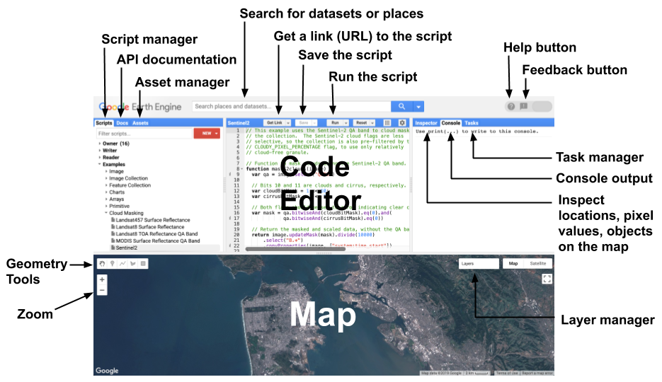
Components of the Earth Engine Code Editor at code.earthengine.google.com
📸 Image Source: Google Earth Engine Guide

💻 JavaScript Code Editor

Central Panel

Acts as the primary space for writing and editing Earth Engine scripts.
Supports ECMAScript 5 (ES5) standards.
Features:
Syntax highlighting for clearer code readability.
Auto-completion for Earth Engine functions and code snippets.
Error detection to help debug code efficiently.

Control Buttons

Run — Executes the current script.
Save — Saves the script to your repository.
Reset — Resets the map and console outputs.
Get Link — Generates a shareable URL of the script environment.

🗺️ Map Display

Visualization Panel

Displays geospatial datasets and script-generated outputs.
Supports multi-layer viewing and comparative analysis.

Layer Management Tools

Adjust layer visibility, transparency, and visualization parameters.
Customize layers using color palettes, gamma, and statistical stretching.

Base Map Options & Drawing Tools

Select from various base maps (satellite, roadmap, terrain, etc.).
Draw geometries directly on the map using tools for points, lines, polygons and rectangles.

📖 Left Panel

Search Bar

Search for datasets, places, and existing scripts.

Docs Tab

Access the complete API reference with searchable documentation.

Scripts Tab

Manage saved, shared, and example scripts using a Git-based system.
Organize scripts into folders and maintain version history.
Full Git integration for external editing.

Assets Tab

Upload and manage custom datasets such as images and tables.
Supports formats like .csv, .tif, and more.

4. 🔍 Right Panel

Inspector Tab

Interactively query map layers.
Displays location coordinates, pixel values, and object properties when clicking on the map.

Console Tab

View script outputs, logs, and printed results.
Interact with objects and charts directly within the console.

Tasks Tab

Manage long-running tasks such as data imports and exports.
Start, monitor, and cancel tasks as needed.

Profiler Tab

Analyze resource consumption (CPU, memory) for script optimization.
Activate via the “Run with profiler” option.

🔗 Script Management

Get Link

Generate snapshot URLs that replicate the script environment for sharing.
Options include:
Hiding code when sharing
Disabling auto-run in shared links

Saved Script Links

Provides stable URLs that always load the latest saved version.
Shareable based on user permissions.

Manage Links

View, remove, and download previously generated links.

Script Modules

Share code between scripts using exports and require functions.
Supports modular development with well-documented modules.

📊 Data Import and Layer Control

Imports Section

Lists all imported datasets and geometry layers.
Options to copy, edit, or delete imports.

Layer Manager

Adjust transparency, visibility, and display settings for each layer.
Customize visualizations using color palettes, gamma, and stretching parameters.

🖌️ Geometry Drawing Tools

Located at the top-left of the map for easy access.
Tools for drawing:
Points
Lines
Polygons
Rectangles
Geometries automatically appear in the Imports section.
Configurable settings for color, geometry type (geometry, feature, or feature collection), and properties.
Lock layers to prevent accidental edits.

📑 Help and Resources

Help Button

Access the Developer’s Guide, community forums, and keyboard shortcuts.
Explore a guided tour of the Code Editor.

Feedback Button

Submit bug reports, feature requests, or suggest new datasets.

📑Working with the JavaScript API: Features and Functionalities

The Earth Engine JavaScript API is the main tool used in the Google Earth Engine (GEE) Code Editor. It helps users work with geospatial data, like satellite images and maps, directly in their browser. Using simple JavaScript code, users can analyze data, create maps, and perform complex calculations without needing powerful local computers.

This API gives access to a huge collection of datasets and allows users to run large-scale analyses quickly by using Google’s cloud servers.
Key Features of the Earth Engine JavaScript API:

🛰️ 1. Massive Data Access: Easily use satellite imagery (like Landsat, MODIS, Sentinel) and geospatial datasets (climate, land cover, etc.)
💻 2. Cloud-Based Processing: Run all computations on Google’s servers, enabling large-scale analysis without needing local resources.
🧭 3. Geospatial Operations: Supports tasks like image classification, time-series analysis, and spatial filtering.
🗺️ 4. Visualization Tools: Visualize data through interactive maps, graphs, and dynamic layers directly in the Code Editor.
📁 5. Incorporate User's Own Datasets: Upload and integrate personal geospatial data for custom analysis.
📤 6. Data Export: Export processed images, tables, or results to Google Drive, Cloud Storage, or Earth Engine Assets for further analysis.

Code example

Here’s an interactive map showcasing India’s surface temperature and elevation using Google Earth Engine. This map combines terrain data with surface temperature analysis and includes a custom legend and time-series chart for deeper insights. You can toggle between layers, switch between satellite imagery, street maps, or street maps with terrain, and zoom in or out to explore the map in detail.

Features Highlighted in This Example:

Multi-layer visualization (Surface Temperature & Elevation)
Custom legends for both layers
Time-series chart of surface temperature (April–June 2023)
Interactive map controls and layer transparency adjustments

Code:

// 1. Define India's geometry using FAO country boundaries
var countries = ee.FeatureCollection('FAO/GAUL/2015/level0');
var india = countries.filter(ee.Filter.eq('ADM0_NAME', 'India')).geometry();
Map.centerObject(india, 4.85); // Center map on India at zoom level 5

// 2. Terrain analysis using SRTM DEM (Only Elevation)
var dem = ee.Image("USGS/SRTMGL1_003").clip(india);

// 3. Surface Temperature using MODIS Land Surface Temperature (LST)
var lst = ee.ImageCollection('MODIS/061/MOD11A2')
  .filterBounds(india) // Filter by India's geometry
  .filterDate('2023-04-01', '2023-06-30') // Date Range (April to June)
  .select('LST_Day_1km') // Select the LST band
  .mean() // Compute the mean LST for the time period
  .multiply(0.02) // Convert to Kelvin using scale factor
  .subtract(273.15) // Convert Kelvin to Celsius
  .rename('LST') // Rename the band to 'LST'
  .clip(india); // Clip to India's geometry

// 4. Visualization parameters
var demParams = {min: 0, max: 4000, palette: ['#006633', '#E5FFCC', '#663300']};
var lstParams = {min: 20, max: 53, palette: ['blue', 'green', 'yellow', 'red']}; // Max Temp set to 53°C

// 5. Add layers to the map
Map.addLayer(dem, demParams, 'Elevation (m)');
Map.addLayer(lst, lstParams, 'Surface Temperature (°C)');

// 6. Create Main Legend Panel (vertical)
var mainLegend = ui.Panel({
  layout: ui.Panel.Layout.flow('vertical'), // Stack legends vertically
  style: {
    position: 'bottom-right',
    padding: '8px',
    backgroundColor: 'white'
  }
});

// ===== Surface Temperature Legend =====
var tempLegend = ui.Panel(); // Panel for temperature legend

// Title
tempLegend.add(ui.Label({
  value: 'Surface Temperature (°C)',
  style: {fontWeight: 'bold', fontSize: '14px', margin: '0 0 4px 0', textAlign: 'center'}
}));

// Gradient Image for Temperature (Horizontal)
var tempGradient = ee.Image.pixelLonLat().select(0)
  .multiply((53 - 20) / 100)
  .add(20);

var tempColorBar = ui.Thumbnail({
  image: tempGradient,
  params: {
    bbox: [0, 0, 100, 10], // Horizontal bar
    dimensions: '200x10',   // Wide and short for horizontal layout
    min: 20,
    max: 53,
    palette: ['blue', 'green', 'yellow', 'red']
  },
  style: {stretch: 'horizontal', margin: '0 auto', maxWidth: '200px'}
});

// Labels for Temperature
var tempLabels = ui.Panel({
  layout: ui.Panel.Layout.flow('horizontal'),
  style: {margin: '4px 0 0 0'}
});
tempLabels.add(ui.Label('20°C', {margin: '0 8px 0 0'}));
tempLabels.add(ui.Label('53°C', {margin: '0 0 0 135px', textAlign: 'right'}));

tempLegend.add(tempColorBar);
tempLegend.add(tempLabels);

// ===== Elevation Legend =====
var elevationLegend = ui.Panel(); // Panel for elevation legend

// Title
elevationLegend.add(ui.Label({
  value: 'Elevation (m)',
  style: {fontWeight: 'bold', fontSize: '14px', margin: '8px 0 4px 0', textAlign: 'center'}
}));

// Gradient Image for Elevation (Horizontal)
var elevationGradient = ee.Image.pixelLonLat().select(0)
  .multiply((4000 - 0) / 100)
  .add(0);

var elevationColorBar = ui.Thumbnail({
  image: elevationGradient,
  params: {
    bbox: [0, 0, 100, 10], // Horizontal bar
    dimensions: '200x10',
    min: 0,
    max: 4000,
    palette: ['#006633', '#E5FFCC', '#663300']
  },
  style: {stretch: 'horizontal', margin: '0 auto', maxWidth: '200px'}
});

// Labels for Elevation
var elevationLabels = ui.Panel({
  layout: ui.Panel.Layout.flow('horizontal'),
  style: {margin: '4px 0 0 0'}
});
elevationLabels.add(ui.Label('0 m', {margin: '0 8px 0 0'}));
elevationLabels.add(ui.Label('4000 m', {margin: '0 0 0 125px', textAlign: 'right'}));

elevationLegend.add(elevationColorBar);
elevationLegend.add(elevationLabels);

// ===== Combine Both Legends =====
mainLegend.add(tempLegend);       // Add Temperature Legend
mainLegend.add(elevationLegend);  // Add Elevation Legend

// Add the combined legend to the map
Map.add(mainLegend);

// 7. Calculate Maximum Surface Temperature
var maxTemp = lst.reduceRegion({
  reducer: ee.Reducer.max(),
  geometry: india,
  scale: 1000,
  maxPixels: 1e13
});

// 8. Print Maximum Temperature
print('Maximum Surface Temperature (°C) from April to June 2023:', maxTemp.get('LST'));

// 9. Plot Time-Series of Surface Temperature over India

// Select MODIS LST ImageCollection again for plotting
var lstCollection = ee.ImageCollection('MODIS/061/MOD11A2')
  .filterBounds(india)
  .filterDate('2023-04-01', '2023-06-30')
  .select('LST_Day_1km')
  .map(function(image) {
    return image.multiply(0.02).subtract(273.15).copyProperties(image, ['system:time_start']);
  });

// Reduce to average temperature over India's geometry
var lstChart = ui.Chart.image.series({
  imageCollection: lstCollection,
  region: india,
  reducer: ee.Reducer.mean(),
  scale: 1000,
  xProperty: 'system:time_start'
})
.setChartType('LineChart')
.setOptions({
  title: 'Surface Temperature Time-Series (April–June 2023)',
  hAxis: {title: 'Date'},
  vAxis: {title: 'Temperature (°C)'},
  lineWidth: 2,
  pointSize: 4,
  colors: ['#d73027']
});

// Print the chart to the console
print(lstChart);
print("The time-series graph shows how the average surface temperature (LST) over India \nchanges between April and June 2023, \nbased on data from the MODIS Land Surface Temperature (LST) product.");

Google Earth Engine Code Editor Interface

Google Earth Engine Code Editor Interface

Google Earth Engine Code Editor Console

Code Editor Console Panel: Outputs & Time-Series Chart

Breakdown of the Code:

1. Defining Geometry Using FAO GAUL Dataset

The code uses the FAO Global Administrative Unit Layers (GAUL) dataset to define the geometry of a specific region. This dataset provides administrative boundaries for countries and regions.

var countries = ee.FeatureCollection('FAO/GAUL/2015/level0');
var region = countries.filter(ee.Filter.eq('ADM0_NAME', 'India')).geometry();
Map.centerObject(region, 4.85); // Center map on the region

Reference

2. Terrain Analysis Using SRTM DEM

The SRTM Digital Elevation Model (DEM) is used to analyze elevation data.

var dem = ee.Image("USGS/SRTMGL1_003").clip(region);

Reference

3. Surface Temperature Calculation Using MODIS LST

The code calculates surface temperature using the MODIS Land Surface Temperature (LST) dataset. MODIS provides daily global temperature data, which is filtered, averaged, and converted from Kelvin to Celsius.

var lst = ee.ImageCollection('MODIS/061/MOD11A2')
  .filterBounds(india) // Filter by India's geometry
  .filterDate('2023-04-01', '2023-06-30') // Date Range (April to June)
  .select('LST_Day_1km') // Select the LST band
  .mean() // Compute the mean LST for the time period
  .multiply(0.02) // Convert to Kelvin using scale factor
  .subtract(273.15) // Convert Kelvin to Celsius
  .rename('LST') // Rename the band to 'LST'
  .clip(india); // Clip to India's geometry

Reference

4. Visualization Parameters The code defines custom visualization parameters for elevation and surface temperature, including color palettes and value ranges. These parameters ensure that the data is displayed clearly and intuitively.

var demParams = {min: 0, max: 4000, palette: ['#006633', '#E5FFCC', '#663300']};
var lstParams = {min: 20, max: 53, palette: ['blue', 'green', 'yellow', 'red']}; // Max Temp set to 53°C

Reference

5. Adding Layers to the Map: The elevation and surface temperature layers are added to the map, allowing users to interactively explore the data.

Map.addLayer(dem, demParams, 'Elevation (m)');
Map.addLayer(lst, lstParams, 'Surface Temperature (°C)');

Reference

6. Creating Custom Legends The code creates interactive legends for both elevation and surface temperature using the ui.Panel and ui.Thumbnail components. These legends provide clear visual cues for interpreting the data.

var mainLegend = ui.Panel({
  layout: ui.Panel.Layout.flow('vertical'),
  style: {
    position: 'bottom-right',
    padding: '8px',
    backgroundColor: 'white'
  }
});

// Temperature Legend
var tempLegend = ui.Panel();
tempLegend.add(ui.Label({
  value: 'Surface Temperature (°C)',
  style: {fontWeight: 'bold', fontSize: '14px', margin: '0 0 4px 0', textAlign: 'center'}
}));

var tempGradient = ee.Image.pixelLonLat().select(0)
  .multiply((53 - 20) / 100)
  .add(20);

var tempColorBar = ui.Thumbnail({
  image: tempGradient,
  params: {
    bbox: [0, 0, 100, 10],
    dimensions: '200x10',
    min: 20,
    max: 53,
    palette: ['blue', 'green', 'yellow', 'red']
  },
  style: {stretch: 'horizontal', margin: '0 auto', maxWidth: '200px'}
});

var tempLabels = ui.Panel({
  layout: ui.Panel.Layout.flow('horizontal'),
  style: {margin: '4px 0 0 0'}
});
tempLabels.add(ui.Label('20°C', {margin: '0 8px 0 0'}));
tempLabels.add(ui.Label('53°C', {margin: '0 0 0 135px', textAlign: 'right'}));

tempLegend.add(tempColorBar);
tempLegend.add(tempLabels);

// Elevation Legend
var elevationLegend = ui.Panel();
elevationLegend.add(ui.Label({
  value: 'Elevation (m)',
  style: {fontWeight: 'bold', fontSize: '14px', margin: '8px 0 4px 0', textAlign: 'center'}
}));

var elevationGradient = ee.Image.pixelLonLat().select(0)
  .multiply((4000 - 0) / 100)
  .add(0);

var elevationColorBar = ui.Thumbnail({
  image: elevationGradient,
  params: {
    bbox: [0, 0, 100, 10],
    dimensions: '200x10',
    min: 0,
    max: 4000,
    palette: ['#006633', '#E5FFCC', '#663300']
  },
  style: {stretch: 'horizontal', margin: '0 auto', maxWidth: '200px'}
});

var elevationLabels = ui.Panel({
  layout: ui.Panel.Layout.flow('horizontal'),
  style: {margin: '4px 0 0 0'}
});
elevationLabels.add(ui.Label('0 m', {margin: '0 8px 0 0'}));
elevationLabels.add(ui.Label('4000 m', {margin: '0 0 0 125px', textAlign: 'right'}));

elevationLegend.add(elevationColorBar);
elevationLegend.add(elevationLabels);

// Combine Legends
mainLegend.add(tempLegend);
mainLegend.add(elevationLegend);
Map.add(mainLegend);

Reference

7. Calculate Maximum Surface Temperature The code calculates the maximum surface temperature within the region using the reduceRegion function. This demonstrates how to extract specific statistics from geospatial data.

var maxTemp = lst.reduceRegion({
  reducer: ee.Reducer.max(),
  geometry: india,
  scale: 1000,
  maxPixels: 1e13
});

Reference

8. Plot Time-Series of Surface Temperature over India This section calculates and visualizes the average surface temperature over India for the period from April to June 2023. Here’s how it works:

Select MODIS LST ImageCollection:

The lst Collection is created by filtering the MODIS LST dataset for India and the specified date range. The LST values are converted from Kelvin to Celsius using .multiply(0.02).subtract(273.15). The system:time_start property is preserved for time-series plotting.

var lstCollection = ee.ImageCollection('MODIS/061/MOD11A2')
  .filterBounds(india)
  .filterDate('2023-04-01', '2023-06-30')
  .select('LST_Day_1km')
  .map(function(image) {
    return image.multiply(0.02).subtract(273.15).copyProperties(image, ['system:time_start']);
  });

Reduce to Average Temperature: The ui.Chart.image.series function calculates the average temperature over India for each image in the collection. The reducer: ee.Reducer.mean() computes the mean temperature for each date.

var lstChart = ui.Chart.image.series({
  imageCollection: lstCollection,
  region: india,
  reducer: ee.Reducer.mean(),
  scale: 1000,
  xProperty: 'system:time_start'
})

Customize the Chart: The chart is set as a LineChart with a title, axis labels, and styling options (e.g., line width, point size, color).

.setChartType('LineChart')
.setOptions({
  title: 'Surface Temperature Time-Series (April–June 2023)',
  hAxis: {title: 'Date'},
  vAxis: {title: 'Temperature (°C)'},
  lineWidth: 2,
  pointSize: 4,
  colors: ['#d73027']
});

Print the Chart: The chart is printed to the console for visualization.

print(lstChart);

Add a Description: A brief description of the time-series graph is printed to explain its significance.

print("The time-series graph shows how the average surface temperature (LST) over India \nchanges between April and June 2023, \nbased on data from the MODIS Land Surface Temperature (LST) product.");

Use Cases

Google Earth Engine (GEE) has enabled large-scale environmental monitoring, conservation efforts, and public health initiatives through its powerful geospatial analysis capabilities.
The Google Earth Engine Code Editor Interface utilizes the JavaScript API to simplify data access, processing, and visualization. It provides researchers, developers, and policymakers with an interactive, browser-based environment to analyze massive geospatial datasets without the need for heavy local computing.
This cloud-powered platform streamlines the development of complex geospatial algorithms, supports real-time data exploration, and enables the creation of dynamic visualizations—all directly within the browser.
Here are a few case studies showcasing the practical applications of Google Earth Engine across diverse fields:

1. 🌳 Global Forest Cover Change
The University of Maryland leveraged GEE to map global forest cover changes over more than a decade, analyzing over 143 billion pixels of Landsat data. What would have taken 15 years on a single computer was completed in days using Earth Engine.

2. 🐅 Tiger Habitat Monitoring
Researchers from the University of Minnesota used GEE to assess habitat loss in endangered tiger reserves across 13 countries. With GEE’s computational power, a process that once took years was finished in under a week.

3. 🦟 Malaria Risk Mapping
UCSF’s Global Health Group developed a tool using GEE to predict malaria outbreaks by integrating local case data with real-time satellite imagery, enabling near real-time disease surveillance.

4. 💧 Global Surface Water Mapping
The European Commission’s JRC used GEE to map changes in global surface water over 30 years, aiding water resource management and disaster preparedness.

5. 🌲 Collect Earth for Land Monitoring
The FAO’s Collect Earth tool, powered by GEE, enables detailed land-use change analysis, helping countries monitor deforestation, land degradation, and agricultural trends.

6. 🗺️ Map of Life
The Map of Life team created an interactive tool for conservators to view and analyze species habitat ranges. By combining data from diverse sources using GEE, the platform pinpoints at-risk species and allows users to adjust parameters to see real-time changes in species distribution and protected habitat areas.

7. 🌲 Global Forest Watch
An initiative by the World Resources Institute, Global Forest Watch uses GEE to monitor deforestation in near real-time. Since its launch in 2014, it has helped corporations, governments, and conservation groups track forest changes and combat illegal logging.

These examples highlight GEE’s versatility in tackling complex environmental and humanitarian challenges at a global scale.

Conclusion

Google Earth Engine (GEE) stands out as a transformative tool for geospatial analysis, enabling users to employ the power of satellite imagery and vast datasets without the need for heavy local computing.
Its browser-based JavaScript API and Code Editor streamline complex geospatial workflows, making it accessible to a wide range of users—from researchers and policymakers to developers and students.

By simplifying data access, processing, and visualization, GEE empowers users to tackle real-world challenges. The platform’s ability to combine historical data with real-time monitoring opens new possibilities for scientific research, environmental conservation, and informed decision-making.

Whether you’re just starting out or diving into complex analyses, Earth Engine offers the tools and resources to turn data into meaningful insights. Explore its vast capabilities, experiment with the Code Editor, and contribute to data-driven solutions for global challenges.

References

1. GEE Official Guides – Comprehensive documentation covering Earth Engine’s features and usage.

2. Code Editor Playground Guide – A guide to using the Earth Engine Code Editor for writing and running JavaScript code directly in the browser.

3. JavaScript Quickstart – A beginner-friendly guide to quickly get started with Earth Engine’s JavaScript API.

4. GEE Account Sign-Up Flow – A step-by-step guide on how to sign up for Google Earth Engine.

5. Earth Engine Case Studies – Explore real-world applications of GEE across environmental, humanitarian, and scientific domains.

6. Earth Engine Platform Overview – Get an overview of Earth Engine’s capabilities and how it works.

7. Earth Engine API Docs – Detailed reference for all classes, methods, and functions in the Earth Engine API.

8. Feature Collections Guide – Learn how to use and manipulate feature collections in Earth Engine.

9. SRTM Digital Elevation Data – Access SRTM DEM data for terrain analysis.

10. MODIS Land Surface Temperature (LST) – Use MODIS data to analyze surface temperatures.

11. Image Visualization Guide – Learn how to style and visualize imagery in Earth Engine.

12. UI Guide – Build interactive user interfaces within the Earth Engine Code Editor.

13. Reducers Introduction – Understand reducers and how to apply them to process geospatial data.

Team

Team J049

Ineesha Sankar - 24110138
Dhulipala Pranathi Mohan - 24110110
Vikram Aditya Dubbaka - 24110385

We would like to thank Professor Nipun Batra for introducing us to Google Earth Engine and providing us the opportunity to work on this assignment. This experience allowed us to explore a new platform and understand process of building our own website and has been a valuable learning experience

Introduction

Installation and Setup

Google Earth Engine Code Editor

📝 Key Components:

💻 JavaScript Code Editor

Central Panel

Control Buttons

🗺️ Map Display

Visualization Panel

Layer Management Tools

Base Map Options & Drawing Tools

📖 Left Panel

Search Bar

Docs Tab

Scripts Tab

Assets Tab

4. 🔍 Right Panel

Inspector Tab

Console Tab

Tasks Tab

Profiler Tab

🔗 Script Management

Get Link

Saved Script Links

Manage Links

Script Modules

📊 Data Import and Layer Control

Imports Section

Layer Manager

🖌️ Geometry Drawing Tools

📑 Help and Resources

Help Button

Feedback Button

📑Working with the JavaScript API: Features and Functionalities

Code example

Features Highlighted in This Example:

Code:

Breakdown of the Code:

Use Cases

Conclusion

References

Further Reading

Team

Team J049